FlexureDiff

Overview

FlexureDiff is a specialized unguided diffusion model for generating compliant mechanism designs, inspired by MIT DeCoDe Lab’s groundbreaking TopoDiff architecture. This model learns the distribution of performant flexure designs and can generate novel, manufacturable flexures from high-level specifications.

The model is trained on a dataset I made of topology-optimized flexure designs designed with my solver spanning various loading conditions and mechanical objectives. Training shows promise and I am making more diffusion models to train diffusion based surrogates to use in my early assembly level generative test formulations.

Note: This research is currently in development and ongoing. Results and methodologies are subject to refinement as the work progresses.

An animation of each denoising step during inference

Technical Implementation

Tech Stack: PyTorch, UNet, TopoDiff, Diffusion Models, Spatial Encoding

Architecture & Training Details

• Model Architecture: Uses TopoDiff UNet architecture for diffusion-based generation
• Data Efficiency: Improved with arbitrary pattern spatially encoded input
• Boundary Conditions: Fixed left side, right side moves in basis directions (translation x, translation y, or rotation z about centroid)
• Load Range: [0.2, 5] mm prescribed displacement
• Design Constraints: 1J max strain energy, 64x64mm design domain

Input Channels

The model processes 5 input channels:

• Strain energy array for solid design domain and the load
• Von Mises stress for solid design domain and the load
• Basis direction for right surface flexibility
• Magnitude of prescribed displacement on the surface
• Normalized ground truth topology array

Dataset

• Training Dataset: 400 topology-optimized flexure samples
• Validation Dataset: 8 sample validation set for feasibility testing

Novel Spatial Encoding

Unlike TopoDiff where loads and boundary conditions are applied at different locations, in FlexureDiff the loads are applied at the same location for every flexure and only varying in magnitude and basis directions.

When using the same location for all prescribed displacement values and simply indicating the direction, the data efficiency was poor. To solve this, I developed a spatial encoding approach using arbitrary patterns to encode the load direction. Each direction receives its own distinct arbitrary pattern, which is then multiplied by the load magnitude. Interestingly, the specific patterns chosen wasn’t important as long as they provide unique spatial signatures for each loading direction.

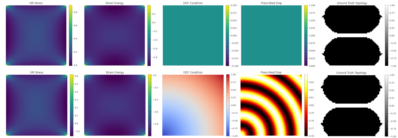
5 inputs for a sample. Top shows normal encoding, bottom shows spatial encoding with arbitrary pattern for translation in the y basis

Without Spatial Encoding

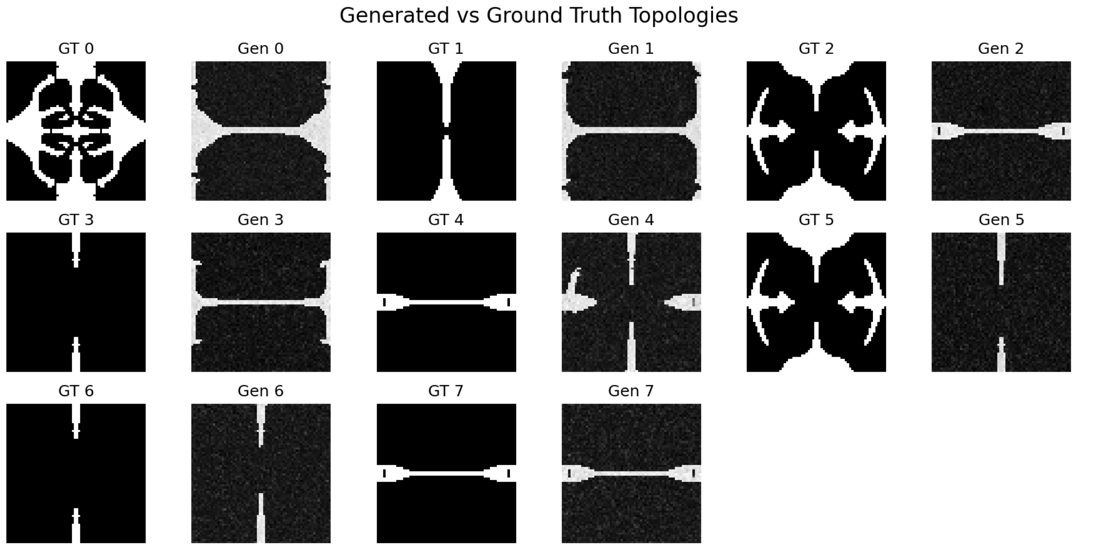
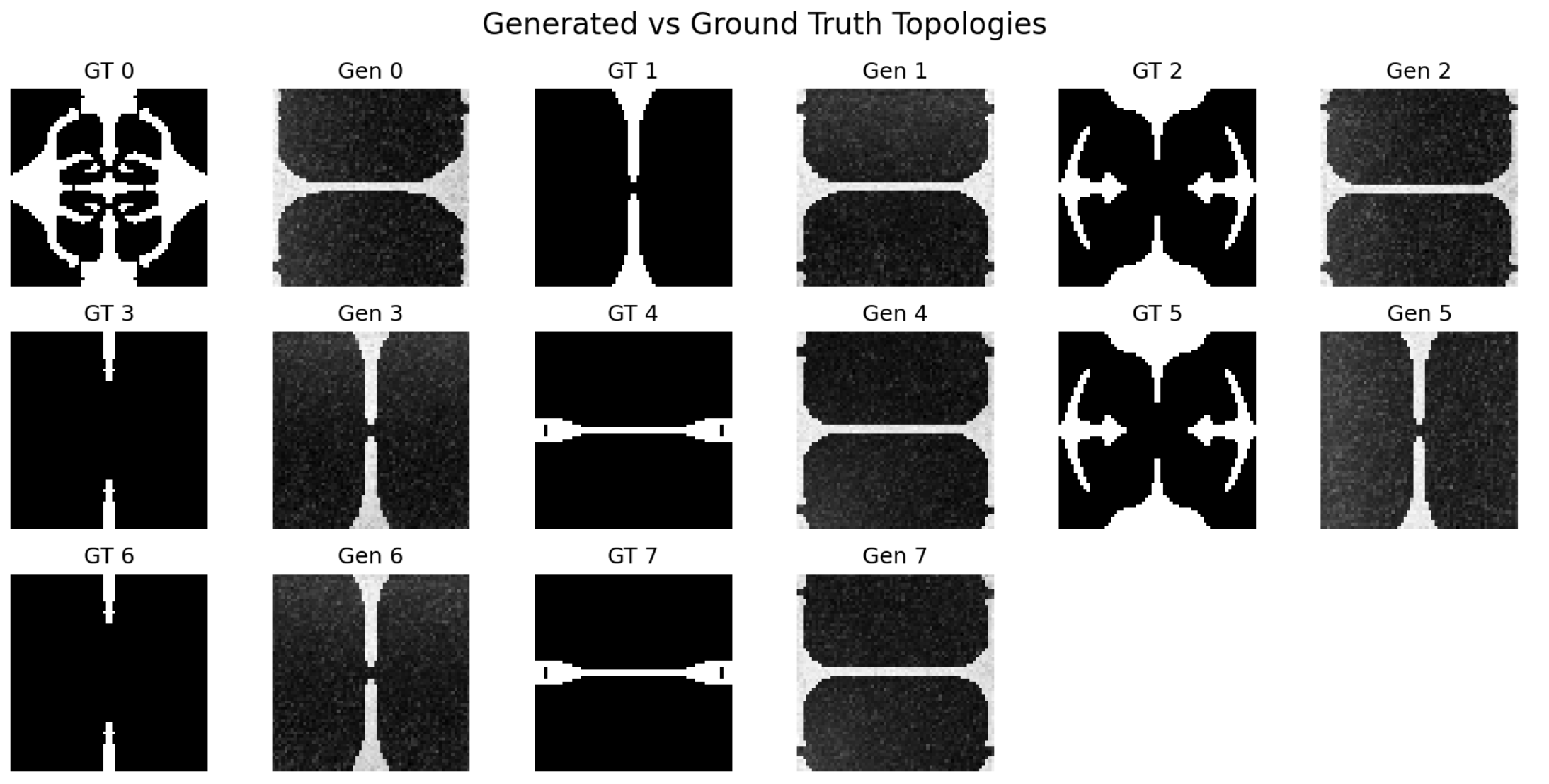
Model evaluation without spatial encoding: Only 3/8 feasible topologies generated after 22,000+ training steps

With Spatial Encoding

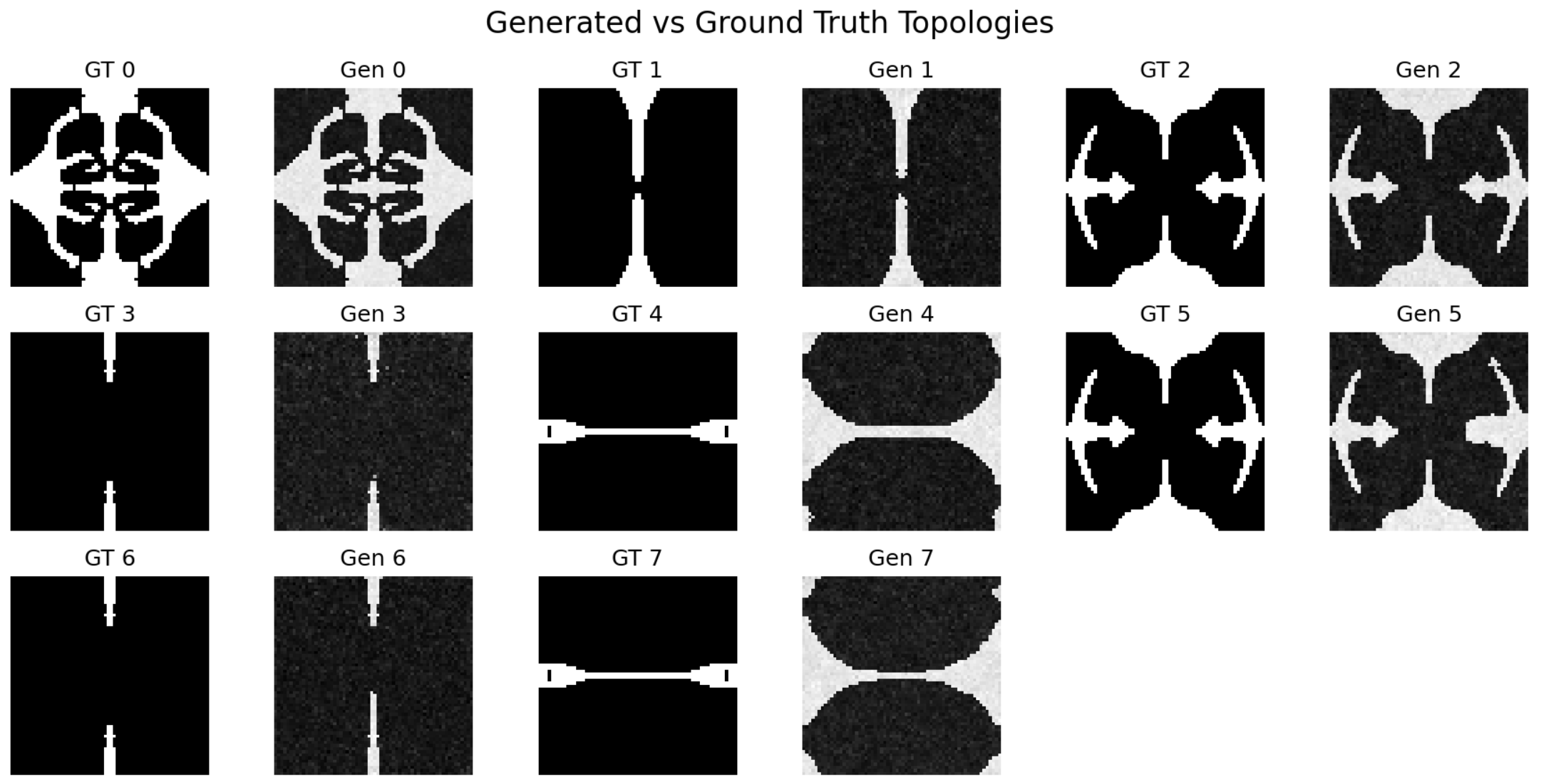
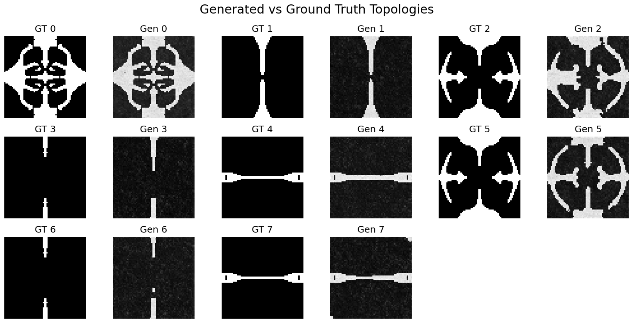
Model evaluation with spatial encoding: 8/8 feasible topologies in only 6,000 steps. Samples 4 and 7 are more feasible/flexible than ground truth and outperform it

The results demonstrate a dramatic improvement: data efficiency increased by more than 3.6x relative to the baseline FlexureDiff model while increasing the feasability of the results by 2.6x. Using the exact same 400-sample dataset and identical hyperparameters on the same model architecture, the spatially-encoded version achieved 100% feasible topology generation (8/8) in just 6,000 training steps, compared to only 37.5% (3/8) feasible topologies after 22,000+ steps without spatial encoding. Note that the evaluation set includes duplicates to verify reproducibility of the generation process.

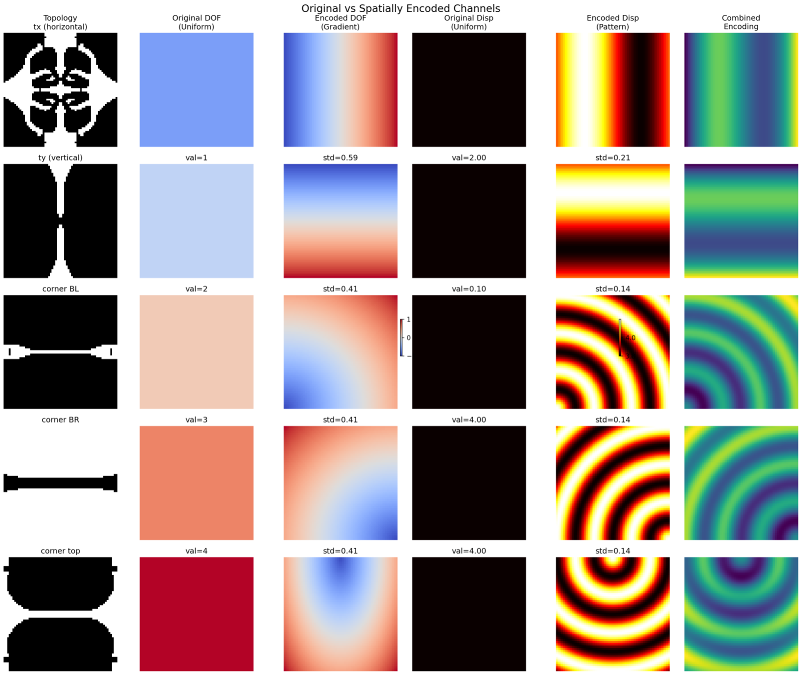
Spatially encoded patterns with arbitrary designs for each DOF

Ablation Study

A larger dataset was used for an ablation study, work in progress. It can be seen that while the loss is about the same between the two groups, the results are dramatically different. Also note that samples 2 and 5 used for evaluation are out of distribution and the rest are in distribution.

With Spatial Encoding

1100_encoding

Without Spatial Encoding

1100_no_encoding

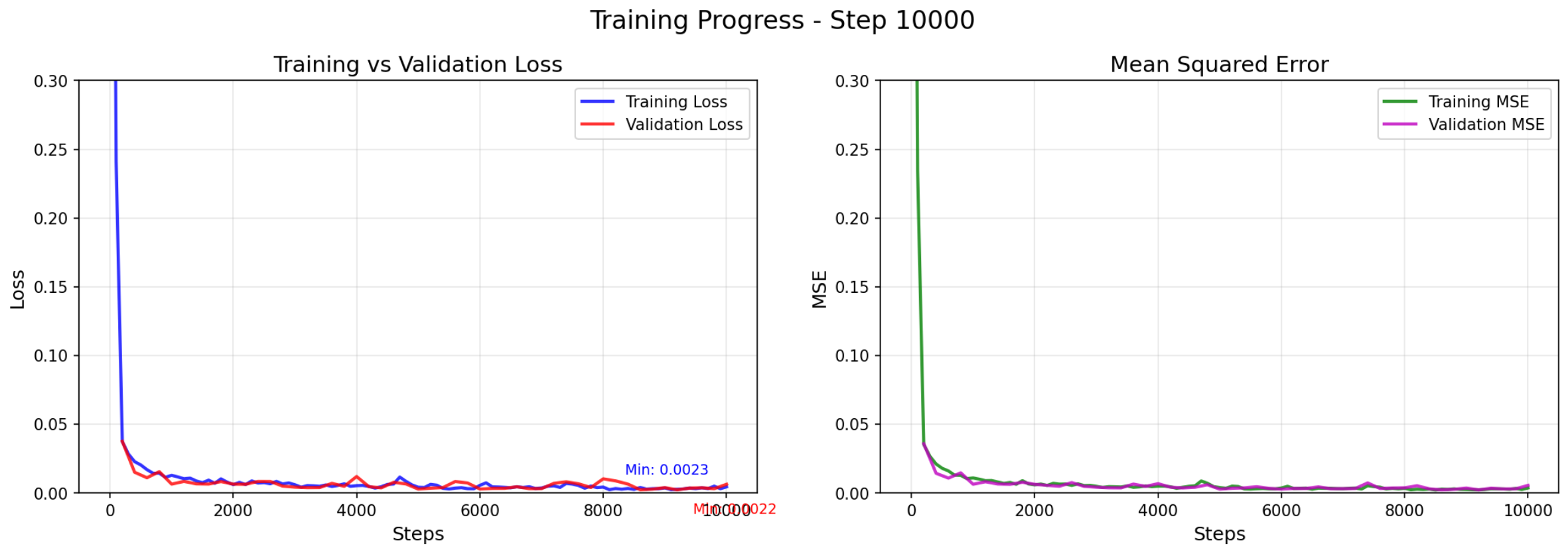
step_10000_encoding

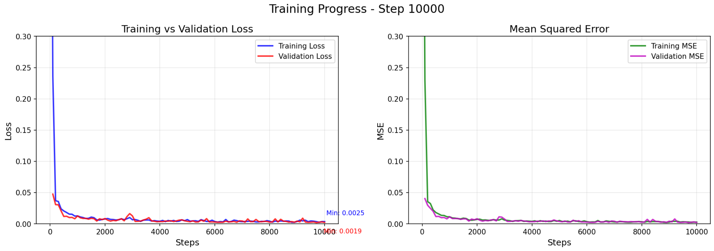
step_10000_no_encoding

Mathematical Formulation

The spatial encoding approach uses two key functions to encode DOF constraints and displacement patterns:

1. DOF Gradient Encoding Function

get_dof_gradient(dof_value, size=64)

Purpose: Generates spatial gradients based on DOF (Degrees of Freedom) condition type

Horizontal ($t_x$, dof_value=0):

$$\text{gradient}(i,j) = \frac{2j}{\text{size}} - 1$$

(linear gradient from -1 to 1)

Vertical ($t_y$, dof_value=1):

$$\text{gradient}(i,j) = \frac{2i}{\text{size}} - 1$$

(linear gradient from -1 to 1)

Corner constraints (dof_value=2,3,4):

$$\text{gradient}(i,j) = 2 \cdot \frac{\sqrt{(x_i - c_x)^2 + (y_j - c_y)^2}}{\sqrt{2}} - 1$$

Where $(c_x, c_y)$ are corner coordinates.

2. Displacement Pattern Encoding Function

get_displacement_pattern(dof_value, base_value, size=64)

Purpose: Generates spatial patterns for prescribed displacement fields

Horizontal ($t_x$, dof_value=0):

$$\text{pattern}(i,j) = \text{base_value} + 0.3 \cdot \sin!\left(\frac{2\pi j}{\text{size}}\right)$$

Vertical ($t_y$, dof_value=1):

$$\text{pattern}(i,j) = \text{base_value} + 0.3 \cdot \sin!\left(\frac{2\pi i}{\text{size}}\right)$$

Corner constraints (dof_value=2,3,4):

$$\text{distance} = \sqrt{(x_i - c_x)^2 + (y_j - c_y)^2}$$

$$\text{pattern}(i,j) = \text{base_value} + 0.2 \cdot \cos(3\pi \cdot \text{distance})$$